Using material fingerprints

In order to use materials data with data analytics and machine learning methods, often it is necessary to encode material properties, like the atomic or electronic structure, typically as vectors of real values. In MADAS, a fingerprint is the combination of a descriptor, i.e., an encoding of material properties, and a similarity measure, i.e., a function that takes two descriptors as arguments and returns their similarity in a range between 0 and 1, where 0 means that both fingerprints are completely dissimilar, and 1 means that they are identical. MADAS allows to compute different built-in fingerprints, as well as supports the creation of custom fingerprints.

In this tutorial you are going to learn how to:

Use built-in fingerprints

Create custom fingerprints

Let’s get started!

Preparations

This tutorial uses a database that was created in the first tutorial “Downloading and managing data with MADAS”. It is suggested to do the tutorials in order, because we will use some functions that are explained in detail in the prior tutorials.

The following lines will create the same data if you didn’t do the first tutorial yet. If you did it already, the data will not be downloaded again.

from madas import MaterialsDatabase

query = {
    "results.material.symmetry.crystal_system:any": [
      "cubic"
    ],
    "results.method.simulation.dft.xc_functional_type:any": [
      "hybrid"
    ],
    "datasets.dataset_name:any": [
      "Materials Database from All-electron Hybrid Functional DFT Calculations"
    ],
    "results.properties.available_properties:all": [
      "dos_electronic"
    ]
  }

db = MaterialsDatabase(filename='materials_database.db')

db.fill_database(query)

2026-04-09 18:37:06,107 - materials_database_log - INFO - Query has already been performed.

The database contains cubic materials from a high-throughput dataset computed using the hybrid HSE06 exchange-correlation functional with density functional theory.

Use built-in fingerprints

First, we are going to use build-in fingerprints to encode the electronic density-of-states (DOS) of these structures.

In the first tutorial, we created a database of these compounds, but currently, the DOS of the compounds is still hidden in the NOMAD archive, and not available as a property directly. We therefore need to find this data and update the database.

Updating the database

First, let’s identity where we can find the DOS in the NOMAD archive.

from madas.utils import print_key_paths

print_key_paths('dos_electronic', db[0].data)

/archive/run/0/calculation/0/dos_electronic
/archive/results/properties/electronic/dos_electronic

We can see that there are two paths, of wich one is in the in the results section. Let’s investigate what is in there.

db[0].get_data_by_path("archive/results/properties/electronic/dos_electronic")

[{'energies': '#/run/0/calculation/0/dos_electronic/0/energies',
  'total': ['#/run/0/calculation/0/dos_electronic/0/total/0'],
  'energy_fermi': -1.1571642761128223e-18}]

We can see that the data here contains paths to the converged total DOS and DOS energies, as well as the Fermi energy. Both paths have a common root. We can investigate what we find there:

db[0].get_data_by_path("archive/run/0/calculation/0/dos_electronic/0").keys()

dict_keys(['n_energies', 'energies', 'energy_fermi', 'energy_ref', 'total', 'species_projected', 'atom_projected', 'orbital_projected', 'fingerprint', 'band_gap'])

In all those keys we can find the information we need to prepare the DOS in a human-readable way:

- total contains the values of the total DOS

- energies contains the energies at which the DOS is evaluated

- energy_ref is a shift that needs to be applied to the energy to shift the energy 0 to the valance band edge for semiconductors, or the Fermi energy for metals

With this information, we can write functions that give us the DOS energies and values from the archive.

Please note that these functions may not work reliably for any selection of data, but are tailored to this example.

from scipy.constants import electron_volt
import numpy as np

from madas import Material

def get_dos_values(material: Material) -> list:
    """
    Get total DOS per unit cell and eV from NOMAD archive dictionary.
    """
    path_ = material.get_data_by_path("archive/results/properties/electronic/dos_electronic/0/total/0")
    dos = np.array(material.get_data_by_path(f'archive{path_[1:]}/value')) * electron_volt
    return dos.tolist()

def get_dos_energies(material: Material) -> list:
    """
    Get DOS energies in eV from a NOMAD archive dictionary, normalized such that E=0 is at the VBM.
    """
    energies_path = material.get_data_by_path("archive/results/properties/electronic/dos_electronic/0/energies")
    energies_ref = f"archive{energies_path[1:]}"
    energies = material.get_data_by_path(energies_ref)
    ref_path = '/'.join(energies_ref.split('/')[:-1]+['energy_ref'])
    ref_energy = material.get_data_by_path(ref_path)
    dos_energies = (np.array(energies) - ref_energy) / electron_volt
    return dos_energies.tolist()

We should test that our functions work:

import matplotlib.pyplot as plt

example_material = db['eNT873N0Cde18DQ6Ni9D5MKpx_7C']

plt.figure(figsize=(10,5))
plt.plot(get_dos_energies(example_material), get_dos_values(example_material))
plt.xlim(-10,10)
plt.ylim(0,60)
plt.xlabel('Energy [eV]')
plt.ylabel('DOS [states/eV/unit cell]')
plt.show()

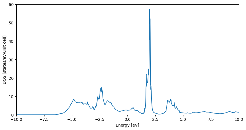
With this we can update the database. Please note that we write the DOS energies and values to the data attribute. This is due to technical reasons, which currently allow only to write scalar quantities or strings to the properties attribute, which may be resolved in the future.

db.update_derived_properties(['dos_values', 'dos_energies'], [get_dos_values, get_dos_energies], target='data')

Now that we have the electronic DOS available, we can use it to compute spectral fingerprints.

Defining and tuning DOS fingerprints

Spectral fingerprints [2] of the electronic DOS are an effective way of describing the electronic structure of materials. They are computed by integrating the DOS over non-uniform energy intervals, that are small close to a chosen reference energy, and get larger as the energy difference to the reference energy increases. This allows to tailor the fingerprint towards a specific energy region of interest. Then, a grid is laid on top of this histogram of states to discretize it. The final fingerprint consists of a vector that represents the colums of the grid, where each grid cell is represented by a 1 if the cell is completely filled by the histogram, or 0 otherwise.

These fingerprints have some parameters that require to be set for each dataset that they are applied to. We will do this in the following.

First, we import the DOSFingerprint class from MADAS:

from madas.fingerprints import DOSFingerprint

To find the right grid parameters for the fingerprint, we start with the default grid:

grid = DOSFingerprint.get_default_grid()

We can inspect what the default settings of the grid are:

grid.resolve_grid_id(grid.grid_id)

{'grid_type': 'nonuniform',
 'e_ref': -2.0,
 'delta_e_min': 0.05,
 'delta_e_max': 1.05,
 'delta_rho_min': 0.5,
 'delta_rho_max': 5.5,
 'width': 7.0,
 'cutoff': [-8.0, 7.0],
 'n_pix': 56}

and plot it for an example entry:

test_fp = DOSFingerprint(grid=grid).calculate(get_dos_energies(example_material), get_dos_values(example_material))

test_fp.plot()

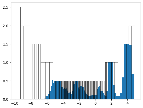
We can see that the grid is well filled, but it looks like the fingerprint would reach the top of the grid in some cases. We can increase the minimal and maximal height of the grid:

grid.n_pix = 2048
grid.delta_rho_min = 5
grid.delta_rho_max = 50

test_fp = DOSFingerprint(grid=grid).calculate(get_dos_energies(example_material), get_dos_values(example_material))
test_fp.plot()

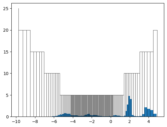
We can see that after our modification, the grid has a lot of space left to account for DOS with many states. With these settings we can compute the fingerprints for all materials. This can be done by iterating over the database:

from madas.utils import tqdm

fps = []
for entry in tqdm(db):
    fp = DOSFingerprint(grid=grid).calculate(entry.data['dos_energies'], entry.data['dos_values'])
    fp.set_mid(entry.mid)
    fps.append(fp)

Because the selection of grid parameters can be challenging for datasets with diverse DOSs, it is useful to check some metrics of the fingerprints. Two examples are the filling factor, which describes how many grid cells are filled:

plt.figure(figsize=(8,5))
plt.hist([fp.filling_factor for fp in fps], bins=50)
plt.show()

We can see that the filling factors are all well below 0.5, so it seems like the grid is able to cover the DOSs well.

Note that for the computation of similarity scores, the empty grid cells are not considered. Therefore it is always better to have more padding.

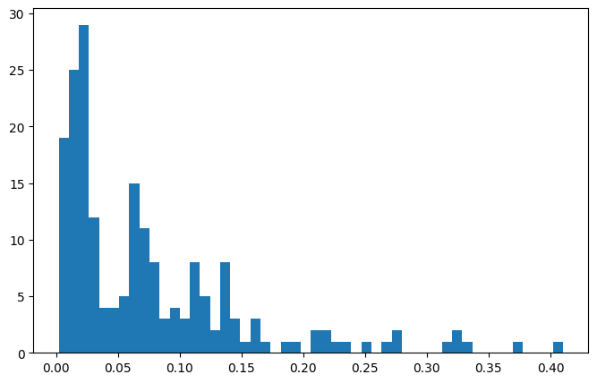
The other metric is overflow, which describes how many states can not be described because they lie outside of the grid.

plt.figure(figsize=(8,5))
plt.hist([fp.overflow for fp in fps], bins=50)
plt.show()

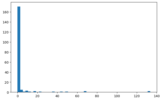
We can see that the vast majority of fingerprints have very low overfow, only some outliers have large values.

We can use these fingerprints now to compute the similarities between materials. For the DOS fingerprints, we use the Tanimoto coefficient [3] as a similarity metric. It describes the similarity between two fingerprints as the overlap between them, divided by the total area covered by combining both fingerprints. The DOSFingerprint has this already implemented, we only need to call the get_similarities function to obtain the similarity scores for a list of fingerprints.

The following plot shows the similarity of the first entry of the database to all other entries:

plt.figure(figsize=(8,5))
plt.scatter(range(len(fps)),fps[0].get_similarities(fps))
plt.xlabel('Database ID')
plt.ylabel('DOS similarity')
plt.show()

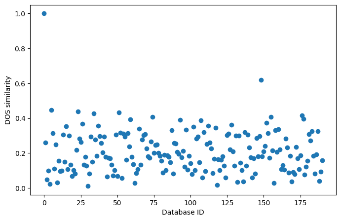
We see that there are no materials that are highly similar to the first entry of the database. As expected, the similarity of the first entry to itself is 1. We could repeat this search for all members of the dataset to discover similar materials, but this is done more efficiently using similarity matrices and clustering. We will explore these in the next tutorial, “Similarity matrices and clustering”.

Lastly, we can add the fingerprints to the database, to retrieve them anytime later, and to avoid having to compute them again. For built-in fingerprints, this can be done by specifying the fingerprint type as a string, and passing the relevant arguments.

db.add_fingerprint('DOS', fingerprint_kwargs={'grid': grid}, energy_path='dos_energies', dos_path='dos_values')

2026-04-09 18:37:44,276 - materials_database_log - INFO - Generating DOS fingerprints...
2026-04-09 18:37:44,278 - materials_database_log - INFO - Generating "DOS" fingerprints.

2026-04-09 18:38:00,204 - materials_database_log - INFO - Writing DOS fingerprints to database...
2026-04-09 18:38:22,401 - materials_database_log - INFO - Finished generation of DOS fingerprints.

Create custom fingerprints

Finally, we can use MADAS to develop, create, and use our own fingerprint types. For this, we will develop a simple descriptor based on the concentrations of the atoms found in the unti cell of a compound. We generate the descriptor, and develop a similarity measure to use alongside with it.

First we develop the descriptor. This is best done on two examples. We pick to specific examples here to illustrate the idea.

example_material = db["dl1IDbhK7pPd2Nlalj1T2zXqP6Xw"]
example_material_2 = db["X8yjRRcfgr2ffZYLelMEVPTLFW-g"]

We find that we can use the Atoms object of a Material to get the atomic numbers Z in a compund:

example_material.atoms.get_atomic_numbers()

array([13, 13, 13, 13, 13, 13, 13, 13, 13, 13, 13, 13, 13, 13, 13, 13, 29,
       29, 29, 29, 29, 29, 29, 29, 29, 29, 29, 29, 29, 29, 29, 29, 29, 29,
       29, 29, 29, 29, 29, 29, 29, 29, 29, 29, 29, 29, 29, 29, 29, 29, 29,
       29])

example_material_2.atoms.get_atomic_numbers()

array([13, 13, 13, 13, 13, 13, 13, 13, 13, 13, 13, 13, 13, 13, 13, 13, 13,
       13, 13, 13, 13, 13, 13, 13, 13, 13, 13, 13, 13, 13, 13, 13, 28, 28,
       28, 28, 28, 28, 28, 28, 28, 28, 28, 28, 28, 28, 28, 28, 28, 28, 28,
       28, 28, 28, 28, 28])

We can see that both structures contain Al (Z=13), but also other elements.

The idea of our custom descriptor is to store the concentrations of each element in the compound. The concentration is the number of atoms of a certain element, divided by the total number of atoms in the unit cell. To represent this quantity for all elements in the unit cell, we could use a vector of lenght 118, with one entry for each element. However, most of these entries will be 0, and we can save memory by storing only these elements that are actually present in the compound. To do so, we can them write the atomic numbers to a dictionary.

We do this individually for each example material:

concentration_dict = {}
for number in example_material.atoms.get_atomic_numbers().tolist():
    try:
        concentration_dict[number] += 1
    except KeyError:
        concentration_dict[number] = 1
for key in concentration_dict.keys():
    concentration_dict[key] /= len(example_material.atoms)

concentration_dict_2 = {}
for number in example_material_2.atoms.get_atomic_numbers().tolist():
    try:
        concentration_dict_2[number] += 1
    except KeyError:
        concentration_dict_2[number] = 1
for key in concentration_dict_2.keys():
    concentration_dict_2[key] /= len(example_material_2.atoms)

concentration_dict

{13: 0.3076923076923077, 29: 0.6923076923076923}

concentration_dict_2

{13: 0.5714285714285714, 28: 0.42857142857142855}

These dictionaries now contain the concentration of each atom type that is present in the compound.

We can create a similarity measure: If we picture the concentrations as a vector, the value in each component is represented by the value of our dictionary. If the dictionary does not have an element as a key, the concentration is 0. The “overlap” between two concentration vectors is then the minimal value for each component of the vector. Since most of the components are 0 anyway, we only need to compare those that exist as keys in the dictionaries. We can use this overlap directly as a similarity measure, as it is naturally defined between 0 and 1.

overlap = 0
for number in concentration_dict.keys():
    try:
        overlap += min(concentration_dict[number], concentration_dict_2[number])
    except KeyError:
        pass

If we look at the concentration dicts above, the lower concentration is found for the first example material. Therefore, the overlap between both should be 0.3076923076923077:

overlap

0.3076923076923077

To compute these fingerprints for all materials in the database, we can write them as a MADAS Fingerprint class:

from madas import Fingerprint

def concentration_vector_similarity(fingerprint1, fingerprint2):
    number_dict1 = fingerprint1.data['concentration_dict']
    number_dict2 = fingerprint2.data['concentration_dict']
    overlap = 0
    for number in number_dict1.keys():
        try:
            overlap += min(number_dict1[number], number_dict2[number])
        except KeyError:
            pass
    return overlap

class ConcentrationVectorFingerprint(Fingerprint):

   # This declaration can be skipped.
   # However, it is advised to explicitly write the `__init__` function.
    def __init__(self,
               name = "ConcentrationVector",
               similarity_function=concentration_vector_similarity,
               pass_on_exceptions=True) -> None:
        super().__init__(name=name,
                         similarity_function=similarity_function,
                         pass_on_exceptions=pass_on_exceptions)

    def calculate(self, atoms):
        concentration_dict = {}
        for number in atoms.get_atomic_numbers().tolist():
            try:
                concentration_dict[number] += 1
            except KeyError:
                concentration_dict[number] = 1
        for key in concentration_dict.keys():
            concentration_dict[key] /= len(atoms)
        # REQUIRED: set the fingerprint data
        self.set_data("concentration_dict", concentration_dict)
        # REQUIRED: return self
        return self

    def from_material(self, material):
        # REQUIRED: set the material identifier for this fingerprint
        self.set_mid(material)
        # calculate the fingerprint
        self.calculate(material.atoms)
        # REQUIRED: return self
        return self

conc_fps = db.get_fingerprints(ConcentrationVectorFingerprint, similarity_function=concentration_vector_similarity)

2026-04-09 18:38:22,569 - materials_database_log - INFO - Generating "<class '__main__.ConcentrationVectorFingerprint'>" fingerprints.

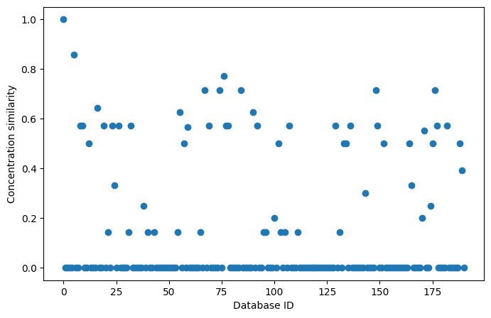
These fingerprints can be used in the same way as built-in fingerprints:

plt.figure(figsize=(8,5))
plt.scatter(range(len(conc_fps)),conc_fps[0].get_similarities(conc_fps))
plt.xlabel('Database ID')
plt.ylabel('Concentration similarity')
plt.show()

We can also add them to the database for later retrieval:

db.add_fingerprint(ConcentrationVectorFingerprint)

2026-04-09 18:38:29,523 - materials_database_log - INFO - Generating ConcentrationVectorFingerprint fingerprints...
2026-04-09 18:38:29,524 - materials_database_log - INFO - Generating "<class '__main__.ConcentrationVectorFingerprint'>" fingerprints.

2026-04-09 18:38:36,020 - materials_database_log - INFO - Writing ConcentrationVectorFingerprint fingerprints to database...
2026-04-09 18:38:57,635 - materials_database_log - INFO - Finished generation of ConcentrationVectorFingerprint fingerprints.

We will see what we can discover in our data with these fingerprints in our next tutorial: “Similarity matrices and clustering”.

References

[1] Akhil S. Nair, Lucas Foppa, and Matthias Scheffler

Materials Database from All-electron Hybrid Functional DFT Calculations.

Sci Data 12, 1518 (2025). https://doi.org/10.1038/s41597-025-05867-z

[2] Martin Kuban, Santiago Rigamonti, Markus Scheidgen, and Claudia Draxl:

Density-of-states similarity descriptor for unsupervised learning from materials data.

Sci Data 9, 646 (2022). https://doi.org/10.1038/s41597-022-01754-z

[3] Peter Willett, John M. Barnard, and Geoffrey M. Downs

Chemical Similarity Searching

J. Chem. Inf. Comput. 38 , 983 996 (1998). https://doi.org/10.1021/ci9800211